Tag Archives: risk

The Effect of ESG Constraints on Systematic Risk

ESG constraints and overlays can create significant systematic exposures within equity portfolios. Whereas some of these exposures may be intentional long and short industry bets, others are unintentional bets on the overall equity market or other macroeconomic factors. In order to deploy ESG strategies successfully, it is vital to identify, quantify, and manage the effect of ESG constraints on systemic risk. That is the only way to avoid unintended hidden risks and the poor performance that results.

Background and Methodology

Over the past decade, institutional investors have been increasingly incorporating Environmental, Social, and Governance (ESG) metrics into their portfolios. Common approaches include separate ESG mandates and ESG constraints applied across entire portfolios. The investors who have implemented these strategies have too often paid little attention to the changes they cause in their portfolios’ factor exposures. This oversight is regrettable, since such changes in systematic risk can dominate subsequent tracking error.

To illustrate a typical ESG overlay effect, we created a constrained portfolio using the FTSE-Russell ESG ratings for S&P 500 Index constituent. The constrained portfolio excluded approximately 18% of the index’s market capitalization with low ESG ratings (below 2.5). A highly predictive multi-factor equity risk model allowed us to analyze the constrained portfolio’s tracking error relative to the unconstrained index.

Tracking Error Due to ESG Constraints

This ESG overlay resulted in an estimated 1.2% tracking error:

The Effect of ESG Constraints on Systematic Risk: Factor and Residual Shares of Tracking Error

Approximately 80% of the tracking error was due to relative factor exposures – relative systematic bets of the constrained portfolio.

Relative Factor Exposures Due to ESG Constraints

Some relative factor bets – for instance, oil price and Energy sector exposures – are reasonable and expected consequences of the overlay. Others look like risky unintended macro tilts:

The Effect of ESG Constraints on Systematic Risk: Key Factors Contributing to Systematic Risk

At nearly 50%, the Equity Market is by far the largest relative factor bet. Market, FX, and Style factor exposures are frequent unintended side-effects of ESG overlays. Fortunately, this risk to strategy’s long-term viability is easy to mitigate. Cheap passive investment vehicles such as index funds, ETFs, futures, and swaps can offset unintended effects of ESG constraints.

The above simple example is representative of the impact of ESG constraints on systematic risk in the real world. Such rules often create factor bets that are undiscovered until they lead to costly underperformance. The effect can be so dramatic that a completely different benchmark could be necessary for this type of strategy. Yet, this solution may not always be feasible and leaves the sacrificed performance unaddressed. Instead, institutions that deploy ESG criteria would benefit from analyzing the resulting exposures and managing any unintended factor bets. Predictive multi-factor models built with liquid investable factors are powerful tools for this task. Such models can identify the inadvertent market bets and guide their mitigation with cheap passive investments, thus avoiding style drift and costly underperformance.

Conclusions

ESG constraints and portfolio overlays can lead to unintended systematic bets.
Some effects of ESG constraints on systematic risk, such as reducing energy sector exposure, may be intentional.
Other effects of ESG constraints may be unintentional long/short market and macro bets.
A robust and predictive equity risk model built with investable factors can identify such unintended effects of ESG constraints and guide their mitigation with cheap and liquid passive instruments.

This article was produced in collaboration among AlphaBetaWorks, a division of Alpha Beta Analytics, LLC, Beacon Pointe, and Peer Analytics.

The information herein is not represented or warranted to be accurate, correct, complete or timely. Past performance is no guarantee of future results. Copyright © 2012-2021, AlphaBetaWorks, Beacon Pointe, and Peer Analytics. All rights reserved. Content may not be republished without express written consent.

The Explanatory Power of Sectors and Style

Leave a reply

Factor analysis is a popular and effective technique that explains and forecasts security returns. The factor models prevalent in academic circles (Fama-French, Carhart) tend to rely heavily on the size and value style factors. Meanwhile, effective industry models often attribute risk to sector and industry factors before style. Which approach is more effective? Though claims that style explains stock returns are common, they usually lack evidence – there is a paucity of research that compares the explanatory power of sectors and style.

This paper provides the missing data and analyzes the explanatory power of sectors and style for U.S. stocks. We find that, after controlling for the market exposure, sectors are slightly more effective than size and approximately four times more effective than value in explaining monthly returns.

Measuring the Explanatory Power of Sectors and Style for U.S. Stock Returns

We analyze the monthly returns of U.S. stocks over the 15-year interval 4/30/2004-4/30-2019. We start with approximately 6,000 stocks that pass minimum market capitalization and liquidity thresholds – a universe similar to the Russell 3000 Index.
For each month in the historical interval and each stock in the sample, we estimate the stock’s market beta.
We calculate (out-of-sample) market residuals (alphas) for a given month using the prior month’s market beta for each stock.
We restrict the analysis to stocks with at least five years of defined market residuals to have a significant sample. This final sample comprises approximately 3,600 stocks.
We construct sector, size, and value factors as follows:
- The sector factors are cap-weighted portfolios of market residuals for the nine sectors equivalent to the top-level GICS sectors.
- The size factor is long the cap-weighted portfolio of stocks in the top 25% and short stocks in the bottom 25%, as ranked by market capitalization.
- The value factor is long the cap-weighted portfolio of stocks in the top 25% and short stocks in the bottom 25%, as ranked by Book/Price.

The results below are insensitive to the specific factor definition and hold across different sector and style portfolios.

For sector, size, and value factors, we regress stocks’ market residuals on the corresponding factor returns and measure each regression’s R². This measures the theoretical (in-sample) explanatory power of sectors and style.
We estimate factor exposures by robust regression. We fit models with iterated re-weighted least squares (IRLS). Observations are exponentially weighted with a half-life of approximately 36-months.

A Comparison of the Explanatory Power of Sectors and Style for U.S. Stock Returns

The chart below plots the distributions of R² from the regressions of U.S. stocks’ market residuals against the sector, size, and value factors. The x-axis plots the intervals of regression R², and the y-axis plots the number of stocks in each interval. Since the distributions approximately follow a power law, we use a log y-axis:

Chart of the explanatory power of sectors, size, and value -- the distributions of the R² (the coefficient of determination) from regressions U.S. stocks’ Market residuals (alphas) on the Sector, Size, and Value Factors — U.S. Stocks: The Distributions of R² for the Regressions of U.S. Stock Market Residuals (Alphas) on the Sector, Size, and Value Factors

The distributions above illustrate the higher explanatory power of sectors compared to style: Whereas sector factors explain over 25% of the variance in market residuals for hundreds of stocks, style factors do so for only a small handful.

The chart below plots the mean R² values:

Chart of the explanatory power of market, sectors, size, and value -- mean R² (the mean coefficient of determination) from regressions U.S. stocks’ returns and Market residuals (alphas) on the Market, Sector, Size, and Value Factors — U.S. Stocks: Mean R² for the Regressions of U.S. Stock Returns and Market Residuals on the Various Factors

Reasons for Sectors’ Higher Explanatory Power

This higher explanatory power of sectors is unsurprising, given that commentary on style performance usually relies on sector factors: “Value underperformed because oil price crashed, and oil producer stocks, which are cheap, suffered.” On the other hand, even the most ideologically pure believer in the primacy of style would not make the statement: “Oil price crashed because oil producer stocks are cheap and value has recently underperformed.” Whereas sector factors can generally explain the reasons for style factor returns, style factors cannot explain the reasons for sector factor returns.

Since style factors capture systematic risk less effectively, portfolio construction from style building blocks can lead to significant unintended exposures. Studies of common smart beta strategies do indeed find such risks and significant market timing. On the other hand, sector and industry exposures offer superior control of systematic risk and more effective building blocks for portfolio construction.

In the sections that follow, we share the statistics on the explanatory power of the various factors.

The Explanatory Power of Market for U.S. Stock Returns

The chart below plots the distribution of R² from the regressions of U.S. stocks’ returns against the Market factor. This step of the analysis allows us to control for market risk and to analyze the explanatory power specific to the other factors:

Chart of the explanatory power of Market -- the distributions of the R² (the coefficient of determination) from regressions U.S. stocks’ returns on the Market Factor — U.S. Stocks: The Distribution of R² for the Regressions of U.S. Stock Returns on the Market Factor

Min.    1st Qu.  Median    Mean    3rd Qu.    Max.
0.0000  0.1117   0.1770    0.1914  0.2563     0.6525

Market explains approximately 20% of the (in-sample) variance of stock returns. The tests below analyze the out-of-sample (investable) market residuals that this step produces.

The Explanatory Power of Sectors for U.S. Stock Returns

The chart below plots the distribution of R² from the regressions of U.S. stocks’ market residuals against sector factors:

Chart of the explanatory power of sectors -- the distributions of the R² (the coefficient of determination) from regressions U.S. stocks’ Market residuals (alphas) on the Sector Factors — U.S. Stocks: The Distribution of R² for the Regressions of U.S. Stock Market Residuals on Sector Factors

Min.    1st Qu.  Median    Mean    3rd Qu.    Max.
0.0000  0.0070   0.0267    0.0618  0.0767     0.6166

For most stocks, sectors explain 2.7% or more of return variance, after controlling for market risk. The average effectiveness is statistically much higher, since sectors explain a large fraction of return variance for some stocks (e.g., Energy sector for Exxon Mobil).

The Explanatory Power of Size for U.S. Stock Returns

The following chart plots the distribution of R² from the regressions of U.S. stocks’ market residuals against the Size factor:

Chart of the explanatory power of size -- the distributions of the R² (the coefficient of determination) from regressions U.S. stocks’ Market residuals (alphas) on the Size Factor — U.S. Stocks: The Distribution of R² for the Regressions of U.S. Stock Market Residuals on the Size Factor

Min.    1st Qu.  Median    Mean    3rd Qu.    Max.
0.0000  0.0089   0.0290    0.0415  0.0599     0.3366

These results support the popularity of the size factor in academic research. For most stocks, the size factor explains 2.9% or more of return variance, after controlling for market risk. Nevertheless, the average explanatory power of sectors is approximately 1.5 times greater.

The Explanatory Power of Value for U.S. Stock Returns

The following chart plots the distribution of R² from the regressions of U.S. stocks’ market residuals against the Value factor:

Chart of the explanatory power of value -- the distributions of the R² (the coefficient of determination) from regressions U.S. stocks’ Market residuals (alphas) on the Value Factor — U.S. Stocks: The Distribution of R² for the Regressions of U.S. Stock Market Residuals on the Value Factor

Min.    1st Qu.  Median    Mean    3rd Qu.    Max.
0.0000  0.0020   0.0092    0.0202  0.0251     0.3350

Contrary to its vogue in academic research, the explanatory power of Value is low, even in these in-sample results. The Value factor explains less than 1% of return variance, after controlling for market risk. Even for the 25% of stocks where the value factor has the greatest explanatory power, it only explains about 2.5% of return variance.

Notes on the Quantitative Methodology

This study controls for market risk before analyzing the explanatory power of sector and style factors. This two-step approach is necessary to avoid the multicollinearity problems that plague academic research into style factors. Since small and large companies typically have different market betas, and since cheap and expensive companies also typically have different market betas, the Fama-French and Carhart factors are collinear. Though this multicollinearity does not necessarily undermine the overall model, it does render individual factor betas and associated statistics meaningless.

We measured the in-sample explanatory power of various factors, similarly to typical academic research on the subject. These results are theoretical and do not represent practically attainable investment outcomes – they are the upper bound for out-of-sample explanatory power: This approach calculates factor exposures and residuals using a regression of stock returns on one or more factors. For instance, the regression of AAPL in the 4-factor Carhart model for 2010-2015 produces betas and alphas that are un-investable. To realize this alpha, one would need to know 2014 returns in order to effectively hedge AAPL in 2010. We use a similar approach in this study, and our analysis suffers from the same limitations – the results are in-sample.

Conclusions

Academic analysis favors factors with less explanatory power than industry’s real-world modeling.
The explanatory power of sectors is slightly higher than that of size, and approximately four times greater than that of value/growth.
Portfolio construction and manager allocation with sector, rather than style building blocks, provide greater control over systematic risk.
Risk models that seek to capture effectively systematic risk should account for sector or industry risk before style risk.
Sectors’ higher explanatory power holds across different industry classifications and style factor definitions.

The information herein is not represented or warranted to be accurate, correct, complete or timely. Past performance is no guarantee of future results. Copyright © 2012-2019, AlphaBetaWorks, a division of Alpha Beta Analytics, LLC. All rights reserved. Content may not be republished without express written consent.

The Predictive Power of Active Share

3 Replies

Active Share is a popular metric that purports to measure portfolio activity. Though Active Share’s fragility and ease of manipulation are increasingly well-understood, there has been no research on its predictive power. This paper quantifies the predictive power of Active Share and finds that, though Active Share is a statistically significant predictor of the performance difference between portfolio and benchmark (there is a relationship between Active Share and how active a fund is relative to a given benchmark), it is a weak one. The relationship explains only about 5% of the variation in activity across U.S. equity mutual funds. The predictive power of Active Share is a small fraction of that achieved with robust and predictive equity risk models.

The Breakdown of Active Share

Active Share — the absolute percentage difference between portfolio and benchmark holdings – is a common metric of fund activity. The flaws of this measure are evident from some simple examples:

If a fund with S&P 500 benchmark buys SPXL (S&P 500 Bull 3x ETF), it becomes more passive and more similar to its benchmark, yet its Active Share increases.
If a fund uses the S&P 500 as its benchmark but indexes Russell 2000, it is passive, yet its Active Share is 100%.
If a fund differs from a benchmark by a single 5% position with 20% residual (idiosyncratic, stock-specific) volatility, and another fund differs from the benchmark by a single 10% position with 5% residual volatility, the second fund is less active, yet it has a higher Active Share.
If a fund holds a secondary listing of a benchmark holding that tracks the primary holding exactly, it becomes no more active, yet its Active Share increases.

Given the flows above, the evidence that Active Share funds that outperform may merely index higher-risk benchmarks is unsurprising.

Measuring Active Management

A common defense is that these criticisms are pathological or esoteric, and unrepresentative of the actual portfolios. Such defense asserts that Active Share measures active management of real-world portfolios.

Astonishingly, we have not seen a single paper assess whether Active Share has any effectiveness in doing what it is supposed to do – identify which funds are more and which are less active. This paper provides such an assessment.

We consider two metrics of fund activity: Tracking Error and monthly active returns (measured as Mean Absolute Difference between portfolio and benchmark returns). Both these metrics measure how different the portfolios are in practice. Whether Active Share measures actual fund activity depends on whether it can differentiate among more and less active funds.

The study dataset comprises portfolio histories of approximately 3,000 U.S. equity mutual funds that are analyzable from regulatory filings. The funds all had 2-10 years of history. Our study uses the bootstrapping statistical technique – we select 10,000 samples and perform the following steps for each sample:

Select a random fund F and a random date D.
Calculate Active Share of F to the S&P 500 ETF (SPY) at D.
Keep only those samples with Active Share between 0 and 0.75. This filter ensures that SPY may be an appropriate benchmark, and excludes small- and mid-capitalization funds that share no holdings with SPY. Such funds would all collapse into a single point with Active Share of 100, impairing statistical analysis.
Measure the activity of F for the following 12 months (period D to D + 12 months). We determine how active a fund is relative to a benchmark by quantifying how similar its performance is to that of the benchmark.

After the above steps, we have 10,000 observations of fund activity as estimated by Active Share versus the funds’ actual activity for the subsequent 12 months.

The Predictive Power of Active Share for U.S. Equity Mutual Funds

The following results quantify the predictive power of Active Share to differentiate among more and less active U.S. equity mutual funds. For perspective, we also include results on the predictive power of robust equity risk models. These results illustrate the relative weakness of Active Share as a measure of fund activity. They also indicate that, far from mitigating legal risk by reliance upon a claimed “best practice,” the use of Active Share to detect closet indexing may instead create legal risk.

The Predictive Power of Active Share to Forecast Future Tracking Error

Although Active Share is a statistically significant metric of fund activity, it is a weak one. Active Share predicts only about 5% of the variation in tracking error across mutual funds:

Residual standard error: 1.702 on 9998 degrees of freedom
Multiple R-squared:  0.05163,   Adjusted R-squared:  0.05154 
F-statistic: 544.3 on 1 and 9998 DF,  p-value: < 2.2e-16

The distributions clearly suffer from heteroscedasticity, which can invalidate tests of statistical significance. To control for this, we also consider the relationship between the rankings of Active Share and future tracking errors. This alternative approach does not affect the results:

Chart of the predictive power of Active Share to forecast future tracking error rank of U.S. equity mutual funds illustrating a weak predictive power. — U.S. Equity Mutual Fund Portfolios: The Predictive Power of Active Share to Forecast Future Tracking Error Rank

Residual standard error: 2811 on 9998 degrees of freedom
Multiple R-squared:  0.05226,   Adjusted R-squared:  0.05217 
F-statistic: 551.3 on 1 and 9998 DF,  p-value: < 2.2e-16

The Predictive Power of Active Share to Forecast Future Active Returns

Active Share also predicts approximately 5% of the variation in monthly absolute active returns across mutual funds:

Chart of the predictive power of Active Share to forecast monthly absolute active return of U.S. equity mutual funds illustrating a weak predictive power. — U.S. Equity Mutual Fund Portfolios: The Predictive Power of Active Share to Forecast Future Active Return

Residual standard error: 0.3986 on 9998 degrees of freedom
Multiple R-squared:  0.04999,   Adjusted R-squared:  0.04989 
F-statistic: 526.1 on 1 and 9998 DF,  p-value: < 2.2e-16

The above results make a generous assumption that all relative returns are due to active management. In fact, much relative performance is attributable to passive differences between a portfolio and a benchmark. We will illustrate this complexity in our follow-up research.

The Predictive Power of Robust Equity Risk Models

To put the predictive power of Active Share into perspective, we compare it to the predictive power of tracking error as estimated by robust and predictive equity risk models. Instead of Active Share, we use AlphaBetaWorks’ default Statistical U.S. Equity Risk Model to forecast tracking error of a fund F at date D.

The Predictive Power of Equity Risk Models to Forecast Future Tracking Error

The equity risk model predicts approximately 38% of the variation in tracking error across mutual funds:

Chart of the predictive power of robust equity risk models to forecast future tracking error of U.S. equity mutual funds illustrating a strong predictive power. — U.S. Equity Mutual Fund Portfolios: The Predictive Power of Robust Equity Risk Models to Forecast Future Tracking Error

Residual standard error: 1.379 on 9998 degrees of freedom
Multiple R-squared: 0.3776, Adjusted R-squared: 0.3776 
F-statistic: 6067 on 1 and 9998 DF, p-value: < 2.2e-16

As with Active Share above, heteroscedasticity does not affect the results. We see a similar relationship when we consider ranks instead of values:

Chart of the predictive power of robust equity risk models to forecast future tracking error rank of U.S. equity mutual funds illustrating a strong predictive power. — U.S. Equity Mutual Fund Portfolios: The Predictive Power of Robust Equity Risk Models to Forecast Future Tracking Error Rank

Residual standard error: 2278 on 9998 degrees of freedom
 Multiple R-squared:  0.3773,    Adjusted R-squared:  0.3772 
 F-statistic:  6058 on 1 and 9998 DF,  p-value: < 2.2e-16

The Predictive Power of Equity Risk Models to Forecast Future Active Returns

The equity risk model predicts approximately 44% of the variation in monthly absolute active returns across mutual funds:

Chart of the predictive power of robust equity risk models to forecast monthly absolute active return of U.S. equity mutual funds illustrating a strong predictive power. — U.S. Equity Mutual Fund Portfolios: The Predictive Power of Robust Equity Risk Models to Forecast Future Active Return

Residual standard error: 0.3068 on 9998 degrees of freedom
Multiple R-squared:  0.4375,    Adjusted R-squared:  0.4374 
F-statistic:  7776 on 1 and 9998 DF,  p-value: < 2.2e-16

Conclusions

Active Share is a statistically significant metric of active management (there is a relationship between Active Share and how active a fund is relative to a given benchmark), but the predictive power of Active Share is very weak.
Active Share predicts approximately 5% of the variation in tracking error and active returns across U.S. equity mutual funds.
A robust and predictive equity risk model is roughly 7-9-times more effective than Active Share, predicting approximately 40% of the variation in tracking error and active returns across U.S. equity mutual funds.
In the following articles, we will put the above predictive statistics into context and quantify how likely Active Share is to identify closet indexers.

U.S. Smart Beta Crowding

4 Replies

Rapid asset flows into smart beta strategies have led to concerns about froth and a vigorous debate among systematic portfolio vendors. At the same time, few discussions of smart beta crowding are burdened by data on the aggregate risk of smart beta strategies. This article attempts to remedy this data vacuum. We survey the risk factors and the stocks responsible for U.S. smart beta crowding. In doing so, we identify the exposures that would benefit the most from further asset flows into smart beta portfolios and those that would suffer the most from any outflows:

The most crowded factor (systematic) exposures are short Size (overweight smaller companies) and short (underweight) Technology Factors.
The most crowded residual (idiosyncratic, or stock-specific) exposures are short (underweight) FAANG stocks.
Exposures to dumb factors account for over 80% of smart beta crowding.

Our findings refute many common beliefs about smart beta crowding.

It follows that the vigorous performance of Technology shares and FAANG stocks specifically has been in spite of, rather than due to, the asset flows into smart beta strategies. Instead, the principal beneficiaries of such inflows and the most crowded smart beta bet have been smaller companies. Smart beta strategies tend to overweight smaller companies relative to the passive (capitalization-weighted) Market Portfolio. Consequently, smaller companies are most at risk should the flows into smart beta reverse. Given its importance, allocators and portfolio managers should pay particular attention to this Size Factor crowding.

Identifying Smart Beta Crowding

This article applied AlphaBetaWorks’ pioneering analysis of Hedge Fund Crowding to U.S. smart beta equity ETFs. We aggregated the Q2 2017 positions of over 300 U.S. smart beta equity ETFs with approximately $700 billion in total assets. We combined all portfolios into a single position-weighted portfolio – U.S. Smart Beta Aggregate (USSB Aggregate). We then used the AlphaBetaWorks (ABW) Statistical Equity Risk Model – an effective predictor of future risk – to analyze USSB Aggregate’s risk relative to the iShares Russell 3000 ETF (IWV) benchmark. The benchmark is a close proxy for the passive U.S. Equity Market portfolio.

We find that a small number of active bets are behind the aggregate risk and performance of U.S. smart beta ETFs. Our analysis assumes that the U.S. smart beta ETF universe is a good proxy for the total smart beta strategy universe. In this case, the analysis captures overall U.S. smart beta crowding.

Factor and Residual Components of U.S. Smart Beta Crowding

USSB Aggregate has approximately 1% estimated future volatility (tracking error) relative to the Market. Over 80% of this relative risk is due to factor exposures, or factor crowding. This high share of factor crowding is consistent with our earlier findings that the bulk of absolute and relative risk of most smart beta ETFs is due to traditional, or dumb, factors such as Market and Sectors:

Chart of the factor (systematic) and residual (idiosyncratic) components of U.S. smart beta crowding on 6/30/2017

Components of U.S. Smart Beta Crowding in Q2 2017

Source	Volatility (ann. %)	Share of Variance (%)
Factor	0.84	82.45
Residual	0.39	17.55
Total	0.92	100.00

Given how close the aggregate smart beta ETF portfolio is to the Market, closet indexing is a concern, especially for diversified smart beta portfolios. The little active risk that remains is primarily due to the two dumb factor exposures discussed below.

U.S. Smart Beta Factor (Systematic) Crowding

The following chart shows the main factor exposures of USSB Aggregate in red relative to U.S. Market’s exposures in gray:

Chart of the factor exposures contributing most to the factor variance of U.S. Smart Beta Aggregate relative to U.S. Market on 6/30/2017

Significant Absolute and Relative Factor Exposures of U.S. Smart Beta Aggregate in Q2 2017

The main active bet of the smart beta universe is short exposure to the Size Factor (overweighting of smaller companies). Thus, smart beta crowding is largely a bet against market-cap weighting and in favor of smaller companies. This crowded bet is the natural consequence of most modified-weighting schemes that de-emphasize larger companies.

Chart of the main contributions to the factor variance of U.S. Smart Beta Aggregate relative to U.S. Market on 6/30/2017

Factors Contributing Most to Relative Factor Variance of U.S. Smart Beta Aggregate in Q2 2017

Factor	Relative Exposure	Factor Volatility	Share of Relative Factor Variance	Share of Relative Total Variance
Size	-5.58	9.62	42.83	35.31
Technology	-6.85	6.39	40.74	33.59
Utilities	1.88	12.72	7.44	6.14
Energy	0.84	13.06	4.73	3.90
Real Estate	0.99	12.40	3.79	3.13
Industrials	1.22	4.72	2.67	2.20
FX	2.49	6.77	2.46	2.03
Materials	0.80	7.88	1.39	1.15
Financials	-1.28	7.90	-1.70	-1.40
Value	-1.08	15.20	-4.04	-3.33

(Relative exposures and relative variance contribution. All values are in %. Volatility is annualized.)

The short Size Factor smart beta crowding accounts for approximately twice the risk of stock-specific crowding. Consequently, smaller companies stand to lose, and larger companies stand to benefit, on average, from smart beta strategy outflows. The short (underweight) Technology bet is nearly as important.

U.S. Smart Beta Residual (Idiosyncratic) Crowding

The remaining fifth of U.S. smart beta crowding as of 6/30/2017 was due to residual (idiosyncratic, stock-specific) risk:

Chart of the main contributors to the residual variance of U.S. Smart Beta Aggregate relative to U.S. Market on 6/30/2017

Stocks Contributing Most to Relative Residual Variance of U.S. Smart Beta Aggregate in Q2 2017

Symbol	Name	Relative Exposure	Residual Volatility	Share of Relative Residual Variance	Share of Relative Total Variance
AAPL	Apple Inc.	-1.43	13.37	24.43	4.29
FB	Facebook, Inc. A	-0.67	24.17	17.39	3.05
AMZN	Amazon.com, Inc.	-0.74	18.23	12.17	2.13
GOOGL	Alphabet Inc. A	-0.52	12.83	3.04	0.53
MSFT	Microsoft Corporation	-0.56	11.78	2.96	0.52
GOOG	Alphabet Inc. C	-0.54	10.72	2.25	0.39
BRK.B	Berkshire Hathaway B	-0.69	7.55	1.82	0.32
BAC	Bank of America Corporation	-0.46	11.08	1.77	0.31
CASH	Meta Financial Group	0.22	22.74	1.68	0.29
NFLX	Netflix, Inc.	-0.11	40.32	1.23	0.21

(Relative exposures and relative variance contribution. All values are in %. Volatility is annualized.)

The main source of residual U.S. smart beta crowding is short (underweight) exposure to AAPL, FB, AMZN, and GOOGL – the principal members of the FAANG club. The Strong performance of these stocks has been despite, rather than due to, flows into smart beta strategies. On a relative basis, FAANGs have suffered from smart beta asset inflows and, all else equal should outperform in the case of outflows from smart beta strategies.

Summary

Factor (systematic) exposures that capture risks shared by many stocks, rather than individual stocks, are responsible for over 80% of U.S. smart beta crowding.
The most crowded smart beta bet is short Size Factor exposure (overweighting of smaller companies). Thus, smaller companies stand to lose from smart beta strategy outflows.
The most crowded residual smart beta bet is short exposure to (underweighting of) FAANG stocks. Therefore, FAANG stocks should be relative beneficiaries of any smart beta outflows.

The information herein is not represented or warranted to be accurate, correct, complete or timely.
Past performance is no guarantee of future results.
Copyright © 2012-2017, AlphaBetaWorks, a division of Alpha Beta Analytics, LLC. All rights reserved.
Content may not be republished without express written consent.

Replicating Fundamental Indexing with Factor Tilts

Leave a reply

The proliferation of smart beta strategies has raised questions about the relationship between the core risk factors that have formed the foundation of quantitative investment analysis for decades and the growing factor zoo of strategies. Whereas some state that “smart beta is the vehicle to deliver factor investing” others argue that “factor tilts are not smart ‘smart beta’”. A central question is how well dumb beta factors such as Market, Sectors/Industries, and Style (Value/Growth, Big/Small) can replicate the zoo’s residents. The answers drive risk modeling, performance evaluation, and portfolio construction. This article studies replicating fundamental indexing with factor tilts over the past ten years and illustrates how well it has worked. We will discuss the other popular smart beta strategies in subsequent articles.

In this 10-year replication example, the reality falls between the extreme viewpoints above:

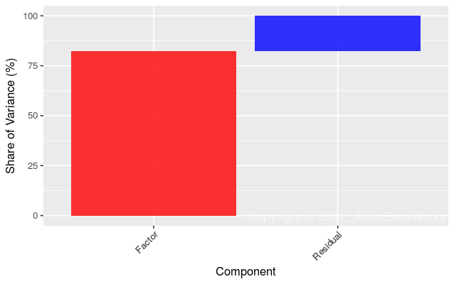
Factor tilts replicate virtually all (>96%) of the absolute variance.
In a typical market environment, factor tilts replicate most (60-75%) of the relative variance. In fact, in this environment, fundamental indexing is substantially replicated with sector rotation. Indeed, most U.S. and international smart beta strategies are largely instances of sector rotation.
In periods of stress, factor tilts fail to replicate the relative variance.
The difference in returns between the target and replicating portfolios is statistically insignificant.
The relative return of the target and replicating portfolios does not follow a random walk – fundamental indexing goes through periods of outperformance and underperformance relative to the replicating portfolio.

We illustrate and quantify the systematic performance that is attainable, and the residual performance that is unattainable, when replicating fundamental indexing with a portfolio of atomic and liquid factor tilts. The replication uses only the rudimentary factors that most commercial equity risk models implement: Market, Sectors, and optionally Style. We also show the environments when replication is more or less successful. It is up to the user to determine whether a given tracking error is adequate for a given application.

Prior Research on Replication

When assumptions and idiosyncrasies of a factor replication exercise are not made explicit, confusion can arise. Any test replicating smart beta with dumb factor tilts is a joint test of the following components:

The equity risk model and the optimizer used to create replicating factor tilt portfolios,
The securities used to implement replicating portfolios,
The portfolio constraints.

Failure of replication based on a flawed model or flawed factors (such as the simple three Fama-French factors suffering from multicollinearity) merely shows the replication process to be flawed; it does not prove the replication impossible.

Replicating Smart Beta Strategies with Dumb Factor Tilts

This article considers fundamental indexing as implemented by the PowerShares FTSE RAFI US 1000 Portfolio (PRF).

We constructed quarterly replicating portfolios using PRF’s position filings. We lagged positions by two months and risk model data by one month to account for filing and processing delays. For example, pre-1/31/2017 PRF positions and 2/28/2017 AlphaBetaWorks U.S. Equity Risk Model were used to construct the 3/31/2017 portfolio, which was next rebalanced on 6/30/2017. The optimizer aimed to minimize estimated future tracking error of the replicating portfolio to PRF, subject to portfolio constraints. Results were unaffected by changes in rebalance delay of a few months.

We attempted to use the simplest replication methodology that is practical and sound. Results vary depending on the security universe, the equity risk model, the optimizer, and the portfolio parameters.

Replicating Fundamental Indexing with Market and Sector Factor Tilts

Market and Sector Factor portfolios were constructed using a Market ETF and nine top-level sector ETFS:

SPY	SPDR S&P 500 ETF Trust
XLY	Consumer Discretionary Select Sector SPDR Fund
XLP	Consumer Staples Select Sector SPDR Fund
XLE	Energy Select Sector SPDR Fund
XLF	Financial Select Sector SPDR Fund
XLV	Health Care Select Sector SPDR Fund
XLI	Industrial Select Sector SPDR Fund
XLB	Materials Select Sector SPDR Fund
XLK	Technology Select Sector SPDR Fund
XLU	Utilities Select Sector SPDR Fund

Position constraint for Sector ETFs was 0 to +100%, and for SPY -100% to +100%. Negative Market weight is necessary to target Market exposures that are not attainable by a long-only portfolio of Sector ETFs. Advanced sector indices, such as the NYSE Pure Exposure Indices, avoid this problem and enable long-only replicating portfolios targeting any combination of exposures.

Fundamental Indexing vs. Market and Sector Tilts: Absolute Performance

The following chart plots cumulative and relative returns for the fundamental indexing portfolio and the replicating Market and Sector Factor portfolio:

Chart of the absolute and relative returns of PowerShares FTSE RAFI US 1000 Portfolio (PRF) and a replicating Market and Sector Factor tilt portfolio

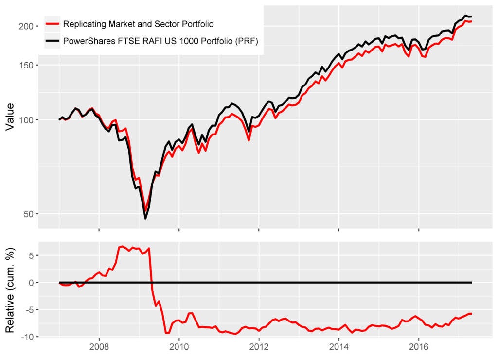
Replicating fundamental indexing with Market and Sector Factor tilts: absolute performance

R-squared       0.9615
Correlation     0.9805
Tracking Error  3.50%

We performed a t-test on the difference in monthly log returns to determine whether they are statistically different from zero:

t = -0.3439
p-value = 0.7315
95 percent confidence interval = (-0.1976, 0.1391)
sample estimate mean = -0.0293

We also performed a Ljung-Box Test on the difference in monthly log returns to determine whether it is a random walk (specifically, whether there are non-0 autocorrelations of the time series):

X-squared = 6.0837
p-value = 0.0136

Though the mean difference in log returns is not statistically different from 0, relative performance is not a random walk. The relative returns of PRF and the replicating portfolio are autocorrelated, as is evident in the chart above.

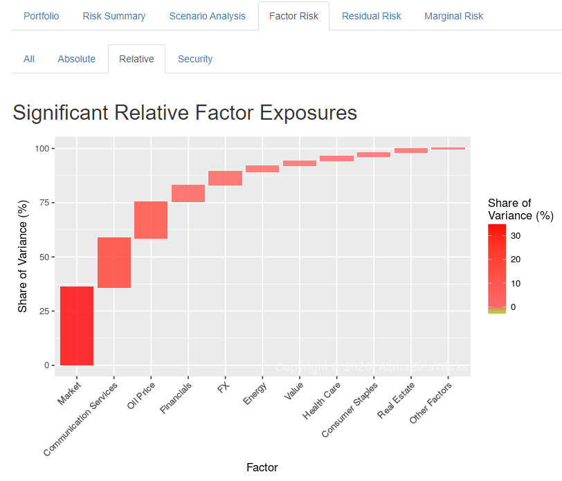
Fundamental Indexing vs. Market and Sector Tilts: Relative Performance

The following chart plots cumulative and relative returns for the fundamental indexing portfolio, the replicating Market and Sector Factor portfolio, and the SPDR S&P 500 ETF (SPY):

Chart of the absolute and relative returns of PowerShares FTSE RAFI US 1000 Portfolio (PRF), a replicating Market and Sector Factor tilt portfolio, and SPDR S&P 500 ETF (SPY)

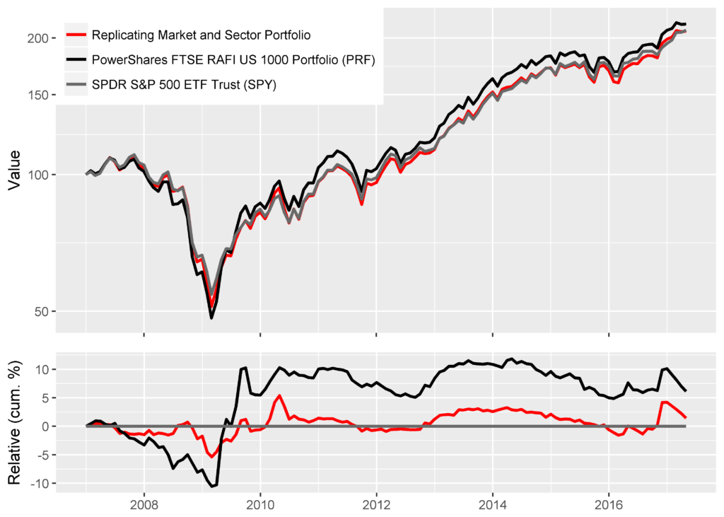
Replicating fundamental indexing with Market and Sector Factor tilts: relative performance

R-squared       0.4929
Correlation     0.7020
Tracking Error  3.50%

Performance difference mostly comes from a few months during the 2008-2009 crisis when residual variance spikes. The replicating portfolio first sharply outperforms and then sharply underperforms. In a calmer environment post-2009, the fit is much closer:

R-squared       0.6124
Correlation     0.7825
Tracking Error  1.75%

Replicating Fundamental Indexing with Market, Sector, and Style Factor Tilts

Market, Sector, and Style Factor tilt portfolios add a Growth/Value ETF pair and a Small-Cap ETF to capture the additional Style Factor exposures:

IWF	iShares Russell 1000 Growth ETF
IWD	iShares Russell 1000 Value ETF
IWM	iShares Russell 2000 ETF

Fundamental Indexing vs. Market, Sector, and Style Tilts: Absolute Performance

The following chart plots cumulative and relative returns for a fundamental indexing portfolio and the replicating Market, Sector, and Style Factor portfolio:

Chart of the absolute and relative returns of PowerShares FTSE RAFI US 1000 Portfolio (PRF) and a replicating Market, Sector, and Style Factor tilt portfolio

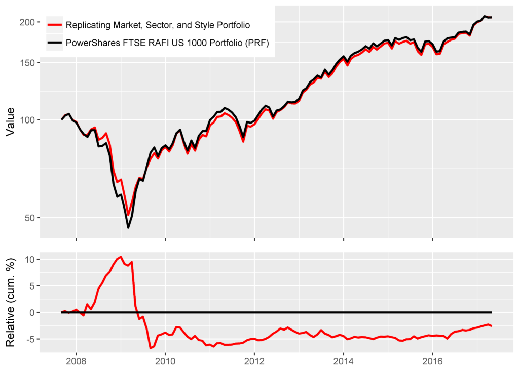
Replicating fundamental indexing with Market, Sector, and Style Factor tilts: absolute performance

R-squared       0.9619
Correlation     0.9807
Tracking Error  3.61%

The t-test results are similar to those of the Market and Sector replicating portfolio:

t = -0.0062504
p-value = 0.995
95 percent confidence interval = (-0.1802, 0.1791)
sample estimate mean = -0.0006

The Ljung-Box test results are also similar:

X-squared = 6.1228
p-value = 0.0134

Fundamental Indexing vs. Market, Sector, and Style Tilts: Relative Performance

The following chart plots cumulative and relative returns for the fundamental indexing portfolio, the replicating Market, Sector, and Style Factor portfolio, and SPY:

Chart of the absolute and relative returns of PowerShares FTSE RAFI US 1000 Portfolio (PRF), a replicating Market, Sector and Style Factor tilt portfolio, and SPDR S&P 500 ETF (SPY)

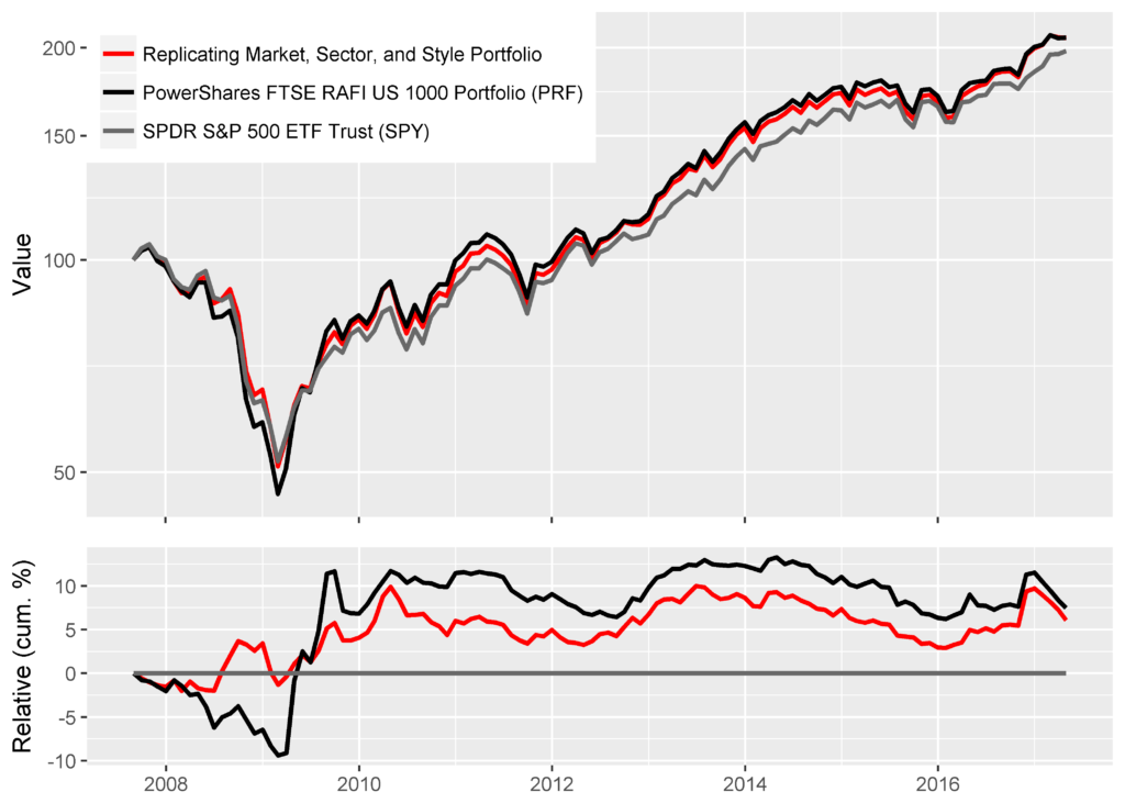
Replicating fundamental indexing with Market, Sector, and Style Factor tilts: relative performance

Over the entire 10-year history, the style factors do not materially change the quality of replication:

R-squared       0.4794
Correlation     0.6924
Tracking Error  3.61%

Post-2009, the style factors do improve the fit:

R-squared        0.7501
Correlation      0.8661
Tracking Error   1.44%

Conclusions

Whether the tracking error of replication is acceptable depends on the application.
Though fully replicating fundamental indexing without any residual tracking error is impossible, even simple Market and Sector factor tilts replicate over 96% of the absolute variance for the fundamental indexing portfolio over the past ten years.
In a normal market environment, factor tilts replicate most (60-75%) of the relative variance for the fundamental indexing portfolio.
In periods of market stress, the tracking error of the replicating portfolio relative to the target is substantial.
The difference in returns between the target and replicating portfolios is statistically insignificant, but it does not follow a random walk and exhibits cycles.

The information herein is not represented or warranted to be accurate, correct, complete or timely.
Past performance is no guarantee of future results.
Copyright © 2012-2017, AlphaBetaWorks, a division of Alpha Beta Analytics, LLC. All rights reserved.
Content may not be republished without express written consent.

What Fraction of International Smart Beta is Dumb Beta?

2 Replies

Though many smart beta ETFs do provide valuable exposures, others mainly re-shuffle familiar dumb beta factors. Our earlier article showed that traditional, or dumb, Market and Sector Betas account for over 92% of monthly return variance for most U.S. equity smart beta ETFs. This article extends the analysis to international smart beta ETFs.

It turns out that international smart beta ETFs are even more heavily dominated by dumb beta factors than their U.S. counterparts. Consequently, rigorous quantitative analysis is even more critical when deploying smart beta strategies internationally. With capable analytics, investors and allocators can detect unnecessarily complex and expensive re-packaging of dumb international factors as smart beta, identify products that do provide unique exposures, and control for unintended international dumb factor exposures.

Measuring the Influence of Dumb Beta Factors on International Smart Beta ETFs

We started with approximately 800 smart beta ETFs. Since our focus was on the broad international equity strategies, we removed portfolios with over 90% invested in U.S. equities and portfolios dominated by a single sector. We also removed portfolios for which returns estimated from historical positions did not reconcile closely with actual returns. We were left with 125 broad international equity smart beta ETFs, covering all the popular international smart beta strategies.

For each ETF, we estimated monthly positions and then used these positions to calculate portfolio factor exposures to traditional (dumb beta) factors such as global Regions (regional equity markets) and Sectors. These ex-ante dumb factor exposures provided us with replicating portfolios composed solely of traditional dumb beta factors. For each international smart beta ETF, we compared replicating portfolio returns to actual returns over the past 10 years, or over the ETF history, whichever was shorter.

The correlation between replicating dumb factor portfolio returns and actual ETF returns quantifies the influence of dumb beta factors on international smart beta ETFs. The higher a correlation, the more similar an ETF is to a portfolio of traditional, simple, and dumb systematic risk factors.

The Influence of Region Beta on International Smart Beta ETFs

Our simplest test used a single systematic risk factor for each security – Region (Region Market Beta). Region Beta measures exposure to one of 10 broad regional equity markets (e.g., North America, Developing Asia). These are the dumbest traditional international factors and also the cheapest to invest in. Since Market Beta is the dominant factor behind portfolio performance, even a very simple model measuring exposures to regional equity markets with robust statistical techniques delivered 0.95 mean and 0.96 median correlations between replicating dumb factor portfolio returns and actual monthly returns for international smart beta ETFs:

Chart of the correlations between returns of replicating portfolios constructed using Region Factors and actual historical returns for over international smart beta equity ETFs

International Smart Beta Equity ETFs: Correlation between replicating Region Factor portfolio returns and actual monthly returns

  Min. 1st Qu.  Median    Mean 3rd Qu.    Max. 
0.6577  0.9390  0.9645  0.9461  0.9818  0.9975

In short: For most broad international smart beta ETFs, Region Market Betas account for at least 93% (0.9645²) of monthly return variance.

The Influence of Region and Sector Betas on International Smart Beta ETFs

We next tested a two-factor model that added Sector Factors. Each security belongs to one of 10 broad sectors (e.g., Energy, Technology). Region and Sector Betas, estimated with robust methods, delivered 0.96 mean and 0.97 median correlations between replicating dumb factor portfolio returns and actual monthly returns for international smart beta ETFs:

Chart of the correlations between returns of replicating portfolios constructed using Region and Sector Factors and actual historical returns for over international smart beta equity ETFs

International Smart Beta Equity ETFs: Correlation between replicating Region and Sector Factor portfolio returns and actual monthly returns

  Min. 1st Qu.  Median    Mean 3rd Qu.    Max. 
0.7017  0.9526  0.9722  0.9578  0.9849  0.9941

In short: For most broad international equity smart beta ETFs, Regional Market and Sector Betas account for over 94% (0.9722²) of monthly return variance. Put differently, only less than 6% of the variance is not attributable to simple Region and Sector factors.

International Smart Beta Variance and International Dumb Beta Variance

Rather than measure correlations between replicating dumb beta portfolio returns and actual ETF returns, we can instead measure the fraction of variance unexplained by dumb beta exposures. The Dumb Beta Variance (in red below) is the distribution of ETFs’ variances due to their dumb beta Region and Sector exposures. The Smart Beta Variance (in blue below) is the distribution of ETFs’ variances unrelated to their dumb beta exposures:

Chart of the percentage of variance explained by traditional, non-smart, or dumb beta Region and Sector Factors and the percentage of variance unexplained by these factors for international smart beta equity ETFs

International Equity Smart Beta ETFs: Percentage of variance explained and unexplained by Region and Sector dumb beta exposures

Percentage of international equity smart beta ETFs’ variances due to dumb beta exposures:

 Min. 1st Qu.  Median    Mean 3rd Qu.    Max. 
49.24   90.74   94.52   91.95   97.00   98.83

Percentage of international equity smart beta ETFs’ variances unrelated to dumb beta exposures:

 Min. 1st Qu.  Median    Mean 3rd Qu.    Max. 
1.174   3.004   5.484   8.052   9.258  50.760

Note that market timing of dumb beta exposures can generate an active return. This return is still due to traditional dumb factor exposures, but it adds value through smart variation in such exposures. Market timing is a relatively small source of return for most international smart beta ETFs and is beyond the scope of this article.

Our analysis excludes Value/Growth and Size Factors, which are decades old and considered dumb beta by some. If one expands the list of dumb beta factors, smart beta variance shrinks further.

Conclusions

Traditional, or dumb, Region and Sector Betas account for over 94% of variance for most international smart beta ETFs.
Smart beta, unexplained by the traditional Region and Sector Betas, accounts for under 6% of variance for most international smart beta ETFs.
With proper analytics, investors and allocators can guard against elaborate re-packaging of dumb international beta as smart beta and spot the products that actually do provide international smart beta exposures.
Investors and allocators can monitor and manage unintended dumb factor exposures of international smart beta portfolios.

The information herein is not represented or warranted to be accurate, correct, complete or timely.
Past performance is no guarantee of future results.
Copyright © 2012-2016, AlphaBetaWorks, a division of Alpha Beta Analytics, LLC. All rights reserved.
Content may not be republished without express written consent.

What Fraction of Smart Beta is Dumb Beta?

Leave a reply

Our earlier articles discussed how some smart beta strategies turn out to be merely high beta strategies, and how others actively time the market, requiring careful monitoring. We also showed that the returns of popular factor ETFs such as Momentum and Quality are mostly attributable to exposures to traditional Market and Sector Factors. We now quantify the influence of traditional factors, or dumb beta, on all broad U.S. equity smart beta ETFs.

Though many smart beta ETFs do provide valuable exposure to idiosyncratic factors, many others mostly re-shuffle exposures to basic dumb factors. To successfully use smart beta products, investors and allocators must apply rigorous quantitative analysis. With capable analytics, they can guard against elaborate (and often expensive) re-packaging of dumb beta as smart beta, identify smart beta products that time dumb beta factors effectively, and monitor smart beta allocations to control for unintended dumb factor exposures.

Measuring the Influence of Dumb Beta Factors on Smart Beta ETFs

We started with approximately 800 U.S. Smart Beta ETFs. Since our focus was on the broad U.S. equity strategies, we removed non-U.S. portfolios and sector portfolios. (Later articles will cover global equity portfolios.) We also removed portfolios for which returns estimated from historical positions did not reconcile closely to reported performance. We were left with 215 broad U.S. equity smart beta ETFs. This nearly complete sample contains all the popular smart beta strategies.

For each ETF, we estimated monthly positions and then used these positions to calculate portfolio factor exposures for traditional (dumb beta) factors such as Market and Sectors. These ex-ante factor exposures can be used to predict or explain the following months’ returns.

The correlation between returns predicted by dumb beta factor exposures and actual returns quantifies the influence of dumb beta factors. The higher the correlation, the more similar a smart beta ETF is to a portfolio of traditional, simple, and dumb systematic risk factors.

The Influence of Market Beta on Smart Beta ETFs

Our simplest test used a single systematic risk factor – Market Beta. This is the dumbest traditional factor and also the cheapest to invest in. Since Market Beta is the dominant factor behind portfolio performance, even a very simple 1-factor model built with robust statistical methods delivered 0.92 mean and 0.94 median correlation between predicted and actual monthly returns for smart beta ETFs:

Chart of the correlations between predicted returns constructed using a single-factor statistical equity risk model and actual historical returns for over 200 U.S. smart beta equity ETFs

U.S. Smart Beta Equity ETFs: Correlation between a single-factor statistical equity risk model’s predictions and actual monthly returns

  Min. 1st Qu.  Median    Mean 3rd Qu.    Max. 
0.5622  0.8972  0.9393  0.9174  0.9693  0.9960

Put differently: For most broad U.S. equity smart beta ETFs, U.S. Market Beta accounts for over 88% of monthly return variance.

The Influence of Market and Sector Betas on Smart Beta ETFs

Since traditional sector/industry allocation is a staple of portfolio construction and risk management, we next tested a two-factor model that added a Sector Factor. Each security belongs to one of 10 broad sectors (e.g., Energy, Technology). Market and Sector Betas, estimated with robust methods, delivered 0.95 mean and 0.96 median correlation between predicted and actual monthly returns for smart beta ETFs:

Chart of the correlations between predicted returns constructed using a two-factor statistical equity risk model and actual historical returns for over 200 U.S. smart beta equity ETFs

U.S. Smart Beta Equity ETFs: Correlation between a two-factor statistical equity risk model’s predictions and actual monthly returns

  Min. 1st Qu.  Median    Mean 3rd Qu.    Max. 
0.5643  0.9320  0.9634  0.9452  0.9805  0.9974

Put differently: For most broad U.S. equity smart beta ETFs, U.S. Market and Sector Betas accounts for over 92% of monthly return variance.

Smart Beta Variance and Dumb Beta Variance

Rather than measuring the correlation between returns predicted by dumb beta exposures and actual returns, we can instead measure the fraction of variance unexplained by dumb beta exposures. This (in blue below) is the fraction of smart beta ETFs’ variance that is unrelated to dumb beta:

Chart of the percentage of variance explained by traditional, non-smart, or dumb beta factors Market and Sectors and the percentage of variance unexplained by these factors for over 200 U.S. smart beta equity ETFs

U.S. Smart Beta Equity ETFs: Percentage of Variance Explained and Unexplained by Dumb Beta Factors

Percentage of Variance Explained by Dumb Beta Factors

Min. 1st Qu.  Median    Mean 3rd Qu.    Max. 
1.85   86.87   92.81   89.71   96.14   99.47

Percentage of Variance Unexplained by Dumb Beta Factors

Min. 1st Qu.  Median    Mean 3rd Qu.    Max. 
 .53    3.86    7.19   10.29   13.13   68.15

Note that some smart beta strategies do provide value by timing the dumb beta factors. This market timing can generate a positive active return, but it still consists of traditional dumb factor exposures and their variation. Market timing by smart beta ETFs is beyond the scope of this article.

The high explanatory power of dumb beta exposures above was achieved with a primitive model using Market and Sector Factors only. If one incorporates Value/Growth and Size factors that are decades old and considered dumb beta by some, smart beta variance shrinks further.

Conclusions

Traditional, or dumb, Market and Sector Betas account for over 92% of variance for most U.S. equity smart beta ETFs.
Smart beta, unexplained by the traditional Market and Sector Betas, accounts for under 8% of variance for most U.S. equity smart beta ETFs.
With proper analytics, investors and allocators can guard against elaborate re-packaging of dumb beta as smart beta.
With proper analytics, investors and allocators can monitor smart beta allocations to control for unintended dumb factor exposures.
Equity risk models can adequately describe and predict the performance of most smart beta strategies with traditional dumb risk factors such as Market and Sectors.

The information herein is not represented or warranted to be accurate, correct, complete or timely.
Past performance is no guarantee of future results.
Copyright © 2012-2016, AlphaBetaWorks, a division of Alpha Beta Analytics, LLC. All rights reserved.
Content may not be republished without express written consent.

Are Momentum ETFs Delivering Momentum Returns?

5 Replies

There is a large difference between momentum strategies in theory and in practice. Given that much of its model performance derives from illiquid securities and high turnover, the academic momentum factor is a theoretical ideal that is not directly investable. Consequently, real-world momentum products, such as momentum ETFs, are restricted to investable liquid securities and usually reduce the approximately 200% annual turnover of theoretical momentum portfolios. After these modifications, their idiosyncratic momentum returns mostly vanish.

We consider a popular momentum ETF and illustrate that its historical performance is almost entirely attributable to passive exposures to simple non-momentum factors, such as Market and Sectors. Investors may thus be able to achieve and even surpass the performance of popular momentum ETFs with transparent, passive, and potentially lower-cost portfolios of simpler funds.

Attributing the Performance of Momentum ETFs to Simpler Factors

We analyzed iShares MSCI USA Momentum Factor ETF (MTUM) using the AlphaBetaWorks Statistical Equity Risk Model – a proven tool for forecasting portfolio risk and performance. We estimated monthly positions from regulatory filings, retrieved positions’ factor (systematic) exposures, and aggregated these. This produced a series of monthly portfolio exposures to simple investable risk factors such as Market, Sector, and Size. The factor exposures at the end of Month 1 and factor returns during Month 2 are used to calculate factor returns during Month 2 and any residual (security-selection, idiosyncratic, stock-specific) returns un-attributable to factors.

There are only two ways for a fund to deviate from a passive portfolio: residual returns un-attributable to factors and factor timing returns due to variation in factor exposures over time. We define and measure both components below.

iShares MSCI USA Momentum Factor (MTUM): Performance Attribution

We used iShares MSCI USA Momentum Factor (MTUM) as an example of a practical implementation of a theoretical momentum portfolio. MTUM is a $1.1bil ETF that seeks to track an index of U.S. large- and mid-cap stocks with high momentum. The fund’s turnover, around 100% annually, is about half that of the theoretical momentum factor.

iShares MSCI USA Momentum Factor (MTUM): Factor Exposures

The following factors are responsible for most of the historical returns and variance of MTUM:

Chart of exposures to the risk factors contributing most to the historical performance of MSCI USA Momentum Factor (MTUM)

MSCI USA Momentum Factor (MTUM): Significant Historical Factor Exposures

	Latest	Mean	Min.	Max.
Market	88.44	84.12	65.46	96.03
Health	23.73	30.28	23.73	34.94
Consumer	74.02	32.53	13.10	74.06
Industrial	1.69	9.71	1.13	24.51
Size	-10.47	-1.04	-11.09	7.67
Oil Price	-2.90	-2.45	-4.94	-0.04
Technology	17.72	16.56	1.50	32.29
Value	-4.86	-2.13	-8.00	5.20
Energy	0.00	1.86	0.00	4.12
Bond Index	6.51	1.08	-22.90	23.64

iShares MSCI USA Momentum Factor (MTUM): Active Return

To replicate MTUM with simple non-momentum factors, one can use a passive portfolio of these simple non-momentum factors with MTUM’s mean exposures as weights. This portfolio defined the Passive Return in the following chart. Active return, or αβReturn, is the performance in excess of this passive replicating portfolio. It is the active return due to residual stock performance and factor timing:

Chart of the cumulative historical active return from security selection and factor timing of MSCI USA Momentum Factor (MTUM)

MSCI USA Momentum Factor (MTUM): Cumulative Passive and Active Returns

MTUM’s performance closely tracks the passive replicating portfolio. Pearson’s correlation between Total Return and Passive Return is 0.96. Consequently, 93% of the variance of monthly returns is attributable to passive factor exposures, primarily to Market and Sector factors.

Once passive exposures to simpler factors have been removed, MTUM’s active return is negligible. Since MTUM’s launch, the cumulative return difference from such passive replicating portfolio has been approximately 1%:

	2013	2014	2015	Total
Total Return	16.73	14.62	8.50	45.18
Passive Return	16.06	16.48	4.55	41.34
αβReturn	1.11	-2.46	2.54	1.12
αReturn	3.91	0.05	0.29	4.27
βReturn	-2.71	-2.52	2.23	-3.05

This active return can be further decomposed into security selection (αReturn) and factor timing (βReturn). These active return components generated low volatility, around 1% annually, mostly offsetting each other as illustrated below:

iShares MSCI USA Momentum Factor (MTUM): Active Return from Security Selection

AlphaBetaWorks’ measure of residual security selection performance is αReturn – performance relative to a factor portfolio that matches the funds’ historical factor exposures. αReturn is the return a fund would have generated if markets had been flat. MTUM has generated approximately 4% cumulative αReturn, primarily in 2013, compared to roughly 1.5% decline for the average U.S. equity ETF:

Chart of the cumulative historical active return from security selection of MSCI USA Momentum Factor (MTUM)

MSCI USA Momentum Factor (MTUM): Cumulative Active Return from Security Selection

iShares MSCI USA Momentum Factor (MTUM): Active Return from Factor Timing

AlphaBetaWorks’ measure of factor timing performance is βReturn – performance due to variation in factor exposures. βReturn is the fund’s outperformance relative to a portfolio with the same mean, but constant, factor exposures as the fund. MTUM generates approximately -3% cumulative βReturn, compared to a roughly 1% decline for the average U.S. equity ETF:

Chart of the cumulative historical active return from factor timing of MSCI USA Momentum Factor (MTUM)

MSCI USA Momentum Factor (MTUM): Cumulative Active Return from Factor Timing

These low active returns are consistent with our earlier findings that many “smart beta” funds are merely high-beta and offer no value over portfolios of conventional dumb-beta funds. It is thus vital to test any new resident of the Factor Zoo to determine whether they are merely exotic breeds of its more boring residents.

Conclusion

Theoretical, or academic, momentum portfolios are not directly investable.
A popular momentum ETF, MSCI USA Momentum Factor (MTUM), did not deviate significantly from a passive portfolio of simpler non-momentum factors.
Investors may be able to achieve and surpass the performance of the popular momentum ETFs with transparent, passive, and potentially lower-cost portfolios of simpler index funds and ETFs.

The information herein is not represented or warranted to be accurate, correct, complete or timely.
Past performance is no guarantee of future results.
Copyright © 2012-2016, AlphaBetaWorks, a division of Alpha Beta Analytics, LLC. All rights reserved.
Content may not be republished without express written consent.

Mutual Fund Closet Indexing: 2015 Update

3 Replies

An index fund aims to track the market or its segment, with low fees. An actively managed fund aims to do better, but with higher fees. So in order to earn its fees, an active mutual fund must take risks. Much of the industry does not even try. Mutual fund closet indexing is the practice of charging active fees for passive management. Over a third of active mutual funds and half of active mutual fund capital appear to be investing passively: Funds tend to become less active as they accumulate assets. Skilled managers who were active in the past may be closet indexing today. Simply by identifying closet indexers, investors can eliminate half of their active management fees, increase allocation to skilled active managers, and improve performance.

Closet Indexing Defined

A common metric of fund activity is Active Share — the percentage difference between portfolio and benchmark holdings. This measure is flawed: If fund with S&P 500 benchmark buys SPXL (S&P 500 Bull 3x ETF), this passive position increases Active Share. If a fund with S&P 500 benchmark indexes Russell 2000, this passive strategy has 100% Active Share. Indeed, recent findings indicate that high Active Share funds that outperform merely track higher-risk benchmarks.

Factor-based analysis of positions can eliminate the above deficiencies. We applied the AlphaBetaWorks Statistical Equity Risk Model to funds’ holdings over time and estimated each fund’s unique factor benchmark. These passive factor benchmarks captured the representative systematic risks of each fund. We then estimated each fund’s past and future tracking errors relative to their factor benchmarks and identified those funds that are unlikely to earn their fees in the future given their current active risk. We also quantified mutual fund closet indexing costs for a typical investor.

This study covers 10-year portfolio history of approximately three thousand U.S. equity mutual funds that are analyzable from regulatory filings. It updates our earlier studies of mutual fund and closet indexing with 2015 data. Due to the larger fund dataset and higher recent market volatility, the mutual fund industry appears slightly more active now than in the 2014 study.

Information Ratio – the Measure of Fund Activity

The Information Ratio (IR) is the measure of active return a fund generates relative to its active risk, or tracking error. We estimated each fund’s IR relative to its factor benchmark. The top 10% of U.S. equity mutual funds achieved IRs above 0.36:

Chart of the historical information ratio for active returns of U.S. mutual funds’ equity portfolios

U.S. Equity Mutual Funds: Historical Information Ratio Distribution

 Min. 1st Qu.  Median    Mean 3rd Qu.    Max.
-5.34   -0.49   -0.22   -0.23    0.06    3.26

If a fund outperforms 90% of the group and achieves 0.36 IR, then it needs tracking error above 1% / 0.36 = 2.79% to generate active return above 1%. So assuming a typical 1% fee, if a fund were able to consistently achieve IR in the 90th percentile, it would need annual tracking error above 2.79% to generate net active return. As we show, much of the industry is far less active. In fact, half of U.S. “active” equity mutual fund assets do not even appear to be trying to earn a 1% active management fee.

Historical Mutual Fund Closet Indexing

Tracking error comes from active exposures: systematic (factor) and idiosyncratic (stock-specific) bets. The AlphaBetaWorks Statistical Equity Risk Model used to estimate these exposures is highly accurate and predictive for a typical equity mutual fund.

Over 28% (746) of the funds have taken too little risk in the past. Even if they had exceeded the performance of 90% of their peers each year, they would still have failed to earn a typical fee. These funds have not even appeared to try to earn their fees:

Chart of the historical mutual fund closet indexing as measured by the tracking error of active returns of U.S. mutual funds’ equity portfolios

U.S. Equity Mutual Funds: Historical Tracking Error Distribution

Min. 1st Qu.  Median    Mean 3rd Qu.    Max.
0.35    2.63    3.95    4.62    5.90   26.60

Current Mutual Fund Closet Indexing

Funds tend to become less active as they grow. To control for this, we estimated current tracking errors of all funds relative to their factor benchmarks.

Over a third (961) of the funds are taking too little risk currently. Even if they exceed the performance of 90% of their peers each year, they will still fail to merit a typical fee. These funds are not even appearing to try to earn their fees:

Chart of the predicted future mutual fund closet indexing as measured by the tracking error of active returns of U.S. mutual funds’ equity portfolios

U.S. Equity Mutual Funds: Predicted Future Tracking Error Distribution

Min. 1st Qu.  Median    Mean 3rd Qu.    Max.
0.92    2.45    3.20    3.52    4.29   20.90

Capital-Weighted Mutual Fund Closet Indexing

Since funds become less active as they grow, larger mutual funds are more likely to closet index. The 36% of mutual funds that have estimated future tracking errors below 2.79% represent half of the assets ($2.25 trillion out of the $4.57 trillion total in our study). Hence, half of active equity mutual fund capital is unlikely to earn a typical free, even when its managers are highly skilled:

Chart of the capital-weighted predicted future mutual fund closet indexing as measured by the tracking error of active returns of U.S. mutual funds’ equity portfolios

U.S. Equity Mutual Funds: Capital-Weighted Predicted Future Tracking Error Distribution

Min. 1st Qu.  Mean 3rd Qu.    Max.
0.92    2.10  2.79    3.72   20.90

Even the most skilled managers will struggle to generate IRs in the 90th percentile each and every year. Therefore, portfolios of large funds, when built without robust analysis of manager activity, may be doomed to negative net active returns. Plenty of closet indexers charge more than the 1% fee we assume, and plenty of investors will lose even more.

A Map of Mutual Fund Closet Indexing

As a manager accumulates assets, fee harvesting becomes more attractive than risk taking. Managers’ utility curves may thus explain large funds’ passivity. The following map of U.S. mutual fund active management skill (defined by the αβScore of active return consistency) and current activity illustrates that large skilled funds are generally less active. Large skilled funds, represented by large purple circles on the right, cluster towards the bottom area of low tracking error:

Chart of the historical active management skill as represented by the consistency of active returns and predicted future tracking error of active returns of U.S. mutual funds’ equity portfolios

U.S. Equity Mutual Funds: Historical Active Management Skill and Predicted Future Activity

In spite of the widespread mutual fund closet indexing, numerous skilled and active funds remain. Many are young and, with a low asset base, have a long way to grow before fee harvesting becomes seductive for their managers.

Conclusions

Over a third of U.S. equity mutual funds are currently so passive that, even if they exceed the information ratios of 90% of their peers, they will still fail to merit a typical fee.
Half of U.S. equity mutual fund capital will fail to merit a typical fee, even when its managers are highly skilled.
As skilled managers accumulate assets, they are more likely to closet index.
A typical investor can re-allocate half of their active equity mutual fund capital to cheap passive vehicles or truly active skilled managers to improve performance.

The information herein is not represented or warranted to be accurate, correct, complete or timely.
Past performance is no guarantee of future results.
Copyright © 2012-2015, AlphaBetaWorks, a division of Alpha Beta Analytics, LLC. All rights reserved.
Content may not be republished without express written consent.

Hedge Fund Closet Indexing: 2015 Update

1 Reply

A fund must take active risk to generate active returns in excess of fees. However, some managers charge active fees but manage their funds passively. Managers also tend to become less active as they accumulate assets. This problem of hedge fund closet indexing is widespread. Over a third of capital invested in U.S. hedge funds’ long equity portfolios is too passive to warrant the common 1.5/15% fee structure, even if its managers are highly skilled. Investors can replace closet indexers with cheap passive vehicles or with truly active skilled managers and improve performance.

Hedge Fund Closet Indexing Background

This article updates our earlier pieces on mutual fund and hedge fund closet indexing with mid-2015 data. We examine current and historical long equity portfolios of approximately 500 U.S. hedge funds that are analyzable from regulatory filings and identify those that are unlikely to earn their fees in the future given their current active risk. We then quantify the cost of hedge fund closet indexing for a typical investor.

Recall from our earlier discussion that Active Share is a brittle metric of fund activity: If a fund buys a position in an index ETF, this passive position may increase Active Share while making the fund less active. If a fund with S&P 500 benchmark simply indexes Russell 2000, this passive fund will have 100% Active Share. These examples are consistent with recent findings that high Active Share funds appear to outperform merely due to miss-specified benchmarks. Our factor-based approach identifies the unique passive factor benchmark for each fund and is free from these deficiencies.

Information Ratio – the Measure of Active Risk Required to Earn a Fee

The Information Ratio (IR) is a measure of active return relative to active risk (tracking error). The best-performing 10% of U.S. hedge funds’ long portfolios achieve IRs above 0.59 relative to their passive factor benchmarks:

Chart of the historical information ratio for active returns of U.S. hedge funds’ long equity portfolios

U.S. Hedge Fund Long Equity Portfolios: Historical Information Ratio Distribution

 Min. 1st Qu.  Median    Mean 3rd Qu.    Max.
-2.58   -0.34   -0.02   -0.04    0.28    2.17

If a fund’s long portfolio exceeds the performance of 90% of the peers and achieves a 0.59 IR, then it needs a tracking error above 1.00% / 0.59 = 1.69% to generate active return above 1%.

Let’s assume that hedge funds’ long equity portfolios are burdened with 1.5% management fee and 15% incentive allocation. Further assuming a 7% market return, the mean fee is 2.55%. If all funds were able to achieve IRs in the 90th percentile, they would need annual tracking error above 2.55% / 0.59 = 4.32% to earn the 2.55% estimated mean fee and a positive net active return. We show below that a significant fraction of the industry takes too little active risk to achieve this tracking error. In fact, much of the industry may not even be trying to earn its fees.

Historical Hedge Fund Closet Indexing

Tracking error comes from funds’ active exposures: systematic (factor) and idiosyncratic (stock-specific) bets. We applied the AlphaBetaWorks Statistical Equity Risk Model to funds’ historical holdings to estimate their unique factor benchmarks. These are passive factor portfolios that capture the representative systematic risks of each fund. We then estimated past and future tracking errors of each fund relative to these benchmarks.

Over 13% (67) of the funds have taken so little risk that, even if they had exceeded the performance of 90% of their peers each year, they would still have failed to earn a typical fee. In other words, these funds have not even appeared to try earning their fees:

Chart of the historical tracking error of active returns of U.S. hedge funds’ long equity portfolios

U.S. Hedge Fund Long Portfolios: Historical Tracking Error Distribution

Min. 1st Qu.  Median    Mean 3rd Qu.    Max.
0.43    6.04   10.04   15.17   19.43  201.00

Estimated Future Hedge Fund Closet Indexing

Fund activity changes over time as managers accumulate assets. Many funds are more passive today than they have been historically. To control for this, we estimated current tracking errors.

Approximately a fifth (88) of the funds are currently taking so little risk that, even if they were to exceed the performance of 90% of their peers each year, they would still fail to merit a typical fee. In other words, these funds are not even appearing to try earning their fees:

Chart of the predicted future tracking error of active returns of U.S. hedge funds’ long equity portfolios

U.S. Hedge Fund Long Portfolios: Predicted Future Tracking Error Distribution

Min. 1st Qu.  Median    Mean 3rd Qu.    Max.
0.76    4.96    7.67   11.01   12.48  148.30

Capital-Weighted Hedge Fund Closet Indexing

Larger hedge funds are more likely to engage in closet indexing. While approximately 20% of hedge funds surveyed have estimated future tracking errors below 4.30%, they represent a third of the assets ($240 billion out of the $720 billion total in our sample). Therefore, a third of hedge fund long equity capital is unlikely to exceed 4.32% tracking error and earn a typical fee, even when its managers are highly skilled:

Chart of the capital-weighted predicted future tracking error of active returns of U.S. hedge funds’ long equity portfolios

U.S. Hedge Fund Long Portfolios: Capital-Weighted Predicted Future Tracking Error Distribution

Min. 1st Qu.  Mean 3rd Qu.    Max.
0.76    3.70  5.49   8.21   116.47

The assumption that all funds will generate higher IRs than 90% of their peers have historically is unrealistic. Hence, a portfolio of large funds built without a robust analysis of hedge fund closet indexing may be doomed to generate negative net active returns, irrespective of the managers’ skills. The 2.55% fee cited here is the estimated mean. Plenty of closet indexers charge more on their long equity portfolios, and plenty of investors who remain with them stand to lose even more.

While there is less closet indexing among hedge funds than among mutual funds, the fees that hedge funds charge and the expectations they set are significantly higher. When practiced by hedge funds, closet indexing is all the more egregious.

A Map of Hedge Fund Closet Indexing

The evolution of managers’ utility curves may explain their reluctance to take risk. As a manager accumulates assets, fee harvesting becomes increasingly attractive. The following map of U.S. hedge fund active management skill and current activity illustrates that large skilled funds are generally less active (large purple circles on the right cluster towards the bottom):

Map of U.S. hedge fund closet indexing for long equity portfolios, charting historical active management skill as represented by the consistency of active returns and predicted future tracking error of active returns of U.S. hedge funds’ long equity portfolios

U.S. Hedge Fund Long Portfolios: Historical Active Management Skill and Predicted Future Activity

Yet, there are notable exceptions – several large, skilled, and active managers remain.

Conclusions

A fifth of U.S. hedge funds’ long equity portfolios are currently so passive that, even if they exceed the information ratios of 90% of their peers, they will still fail to merit a typical fee.
A third of U.S. hedge funds’ long equity capital will fail to merit a typical fee, even when its managers are highly skilled.
As skilled managers accumulate assets, they are more likely to closet index.
A typical hedge fund investor can replace a third of long hedge fund capital with cheap passive vehicles or truly active skilled managers and improve performance.

The information herein is not represented or warranted to be accurate, correct, complete or timely.
Past performance is no guarantee of future results.
Copyright © 2012-2015, AlphaBetaWorks, a division of Alpha Beta Analytics, LLC. All rights reserved.
Content may not be republished without express written consent.